Predictability of the atmospheric state
All the researches in the numerical modeling are motivated by a same reason: giving even more reliable weather forecasts. The importance of the dynamical core and the discretization became obvious at the generalities of ALADIN and AROME. The details of initial condition generation were described at the part of data assimilation. At the physical parametrization part there are methods which count the effect of processes which are smaller than the grid scale of the model. Despite of all the scientific results which were produced on the above mentioned topics the predictability of the weather is still really limited. Meteorologists are not able to predict for any time-range with a sufficient reliability. The model forecasts are always ruled by model errors which have theoretically two main types:
The first is the so called “man made error”. This expression emphasizes that the models are always created by people and will never be able to estimate the complexity of the nature on a perfect way. In modeling the discretization is basically a simplification which is a kind of uncertainty in the prediction. At the data assimilation part it could be seen that initial conditions are never perfectly known. Additionally parametrization methods are not able to describe all physical processes without any simplification. The mentioned sources of the error are the results of the limited knowledge and resources of people.
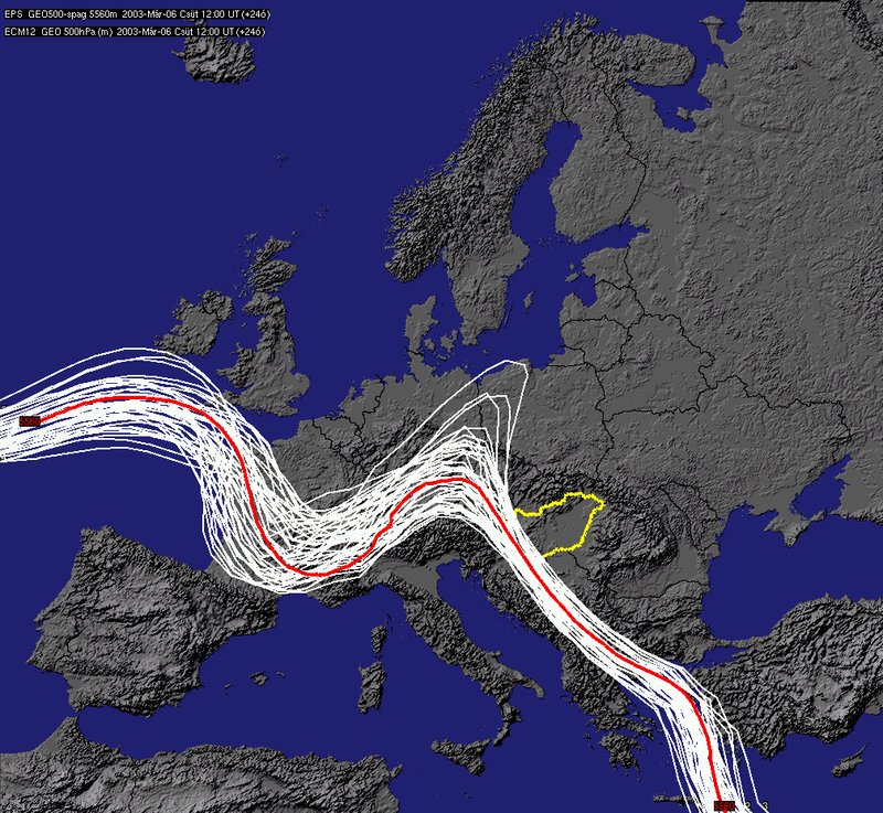
The second big type of errors is the so called “God given error”. For the better understanding it is worth to examine the nature of simple chaotic systems. It could be seen that even the one-dimensional systems which are driven by nonlinear equation can show extreme sensitivity to their initial conditions: a small uncertainty at the beginning of forecast-range can result a big differences later. The atmospheric models are surely not simple systems described by nonlinear partial differential equations and have sometimes millions of variables. These complex systems have the same chaotic behave than the simple nonlinear ones, so they are also very sensitive on their initial conditions. The source of this sensitivity and the caused errors are finally the results of the nature of the atmospheric predictions.
 |
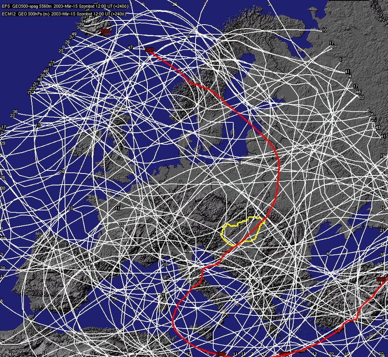 |
The isolines of forecasts started from very similar initial conditions after 24 (left) and 240 (right) hours
Ensemble forecasts
The above mentioned details about the model error can lead to a question: How could we manage the limitations of predictability in the atmosphere? If it is impossible to give a reliable yes/no forecast for the precipitation existence for many days ahead to a certain location, than is there any information which could be presented to the public users? A possible solution for this problem could be the generation of ensemble forecasts and the presentation of the probabilistic information.
In practice ensemble systems always contain more model forecasts which run on a parallel way. These forecasts differ just on small details from each other. The source of the differences could be a perturbation which is added to the initial condition or generated by different settings of physical parametrizations during the model integration. Additionally in limited area models like ALADIN - which is used at OMSZ to produce probabilistic forecasts – global models are needed to have lateral boundary conditions. Perturbations could arrive through these boundary conditions as well. The following table contains the most relevant methods of perturbation generation:
|
Singular vectors |
Singular vectors method help to find a perturbation which evolution is the fastest in accordance with a given norm at the early stage of the forecast. This perturbation can represent the biggest part of the uncertainty in the initial fields at the first stage of the forecast. |
|
Breeding method |
In breeding method random perturbations are added to the forecasts, which can evolve with time. Because of this evolution they are rescaled after a given time. With the rescaled perturbation a new forecast is started, so a cycle is created where the rescaled perturbations always represent such a direction of initial state which contains the biggest part of the uncertainty coming from the previous forecast. This cycle can ‘breed’ the perturbations which is the origin of the name of the method. |
|
Ensemble data assimilation |
At the use of this system more data assimilation cycles are run on a parallel way. The observations are randomly perturbed and used int the different cycles, so more initial conditions are generated. The differences between these initial conditions are the perturbations which represent the most uncertain directions of the analysis. |
|
Multi-model ensemble |
The multi-model ensemble is a simple method. More forecast center have their own deterministic prediction which could be shared with each other and they can be used as an ensemble altogether. |
|
Multi-physics |
Multi-physics is a method to take into account the uncertainty of the physical parametrizations. More physical packages can be used or applied with different settings on a parallel way. |
|
Stochastic physics |
The method of stochastic physics aims the estimation of the uncertainty of parametrization. Random perturbations are added to tendencies which are calculated in the different parametrization schemes. |
|
Dynamical adaptation of global ensemble systems |
Regional forecasts need initial and lateral boundary conditions. From these conditions the perturbations of the global system can penetrate into the local model. These perturbations are the characteristics of the uncertainty of the driving model. |
Regional ensemble prediction system at the Hungarian Meteorological Service
The regional ensemble system of OMSZ contains 11 members which have their initial and lateral boundary conditions from the French global ensemble system (called PEARP). In this global system the singular vectors method is combined with ensemble data assimilation. Multi-physics approach is used to estimate the uncertainty of the parametrizations. In the regional system no local perturbations are added, although there are experiments aiming this goal. Ensemble forecasts start at 18UTC every day and run for +60 hours over a domain covering the continental Europe.
Visualization of the ensemble forecasts
It is not enough to run an ensemble of the forecasts but it is important to visualize the system on a suitable way. In the case of ensemble predictions the visualization method are different then the ‘classical’ ones at deterministic forecasts. All information is needed from the individual forecasts but plots have to keep their persistent and brief style. For example it is impossible to look all details of 11 members with the same accuracy then an individual forecast. The following methods could be used to visualize ensemble forecasts. The examples are from the own regional ensemble forecast and visualization system of OMSZ.
- Visualization of ensemble mean
A possible way is to visualize the mean of the ensemble members which is a similar aspect used at deterministic forecasts. This method needs care because for example one part of the members can show low-pressure and other part can show high-pressure which case produces a plain mean forecast which was not the part of any individual member. - Stamp diagram
The prediction of the individual members can be visualize next to each other for a given parameter and timestep on a decreased size. Stamp diagram help to identify the most relevant characteristic differences but do not allow to see the smaller details because of the smaller size.
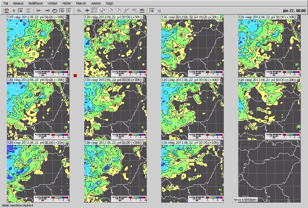
The visualization of regional ensemble system of OMSZ by a stamp diagram of the precipitation
connected to a cold front which arrived Hungary on the night of 22nd of June, 2012
- Plume diagram
Plume diagram is a method to visualize the members together for a given parameter at a given place as a function of time. It shows information about the uncertainty of the forecast and the predictability of the parameter in the actual weather situation.
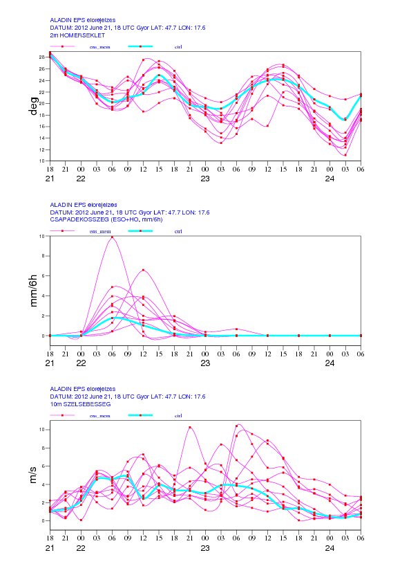
A plume diagram for Győr from the regional ensemble system started at 18 UTC
on 21st of June, 2012. The following parameters can be seen:
2 meter temperature (above), precipitation (middle), wind speed (bottom)
- Probability maps
These maps visualize the probability of a certain event (for example temperature below 0 degree). The probability is determined by the percentage of the members which forecast the occurrence of the event.
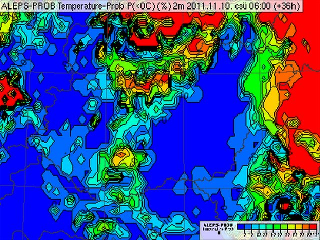
The probability of temperature below 0 degree in the regional ensemble system of OMSZ;
the plot shows the dawn of 10th of November, 2011;
red color belongs to the 100% of possibility and blue to 0%
References
- Hágel, E. and Horányi, A. 2006. The development of a limited area ensemble prediction system at the Hungarian Meteorological Service: sensitivity experiments using global singular vectors, preliminary results. Időjárás 110, 229–252.
- Hágel, E. and Horányi, A. 2007. The ARPEGE/ALADIN limited area ensemble prediction system: the impact of global targeted singular vectors. Meteorologische Zeitschrift 16(6), 653–663.
- Horányi A., Mile M., Szűcs M., 2011: Latest developments around the ALADIN operational short-range ensemble prediction system in Hungary, Tellus, 63A, 642-651